In this video I explain the sampling distribution of the mean, a comparison distribution for thinking about the probability of different mean values selected from a population. I explain how the Central Limit Theorem allows us to infer characteristics of this distribution, and how the variance and standard error can be calculated based on the population variance and the sample size. The sample size influences our level of uncertainty around the population mean and the probability of getting particular means for a sample, and this can be reported by providing the SE or SEM (standard error of the mean) and using error bars in graphs of data. This illustrates why the mean is such a valuable statistic and why interval and ratio level data allow for more robust statistical analyses.

Video Transcript:

Hi, I’m Michael Corayer and this is Psych Exam Review. In the previous videos related to null hypothesis significance testing we’ve had this idea that we look for a comparison distribution, and this is a distribution of a calculation or a test statistic that allows us to assess the probability of getting certain results when the null hypothesis is true. And so now we’re going to look at a particular comparison distribution, and this is a common and fairly important one, and that’s the distribution of the possible averages that we might get if we draw a sample from the population. And this is known as the sampling distribution of the mean.

If we have a population of individual scores and then we randomly select a sample from that population, the sample that we get is not going to perfectly represent the population. It might have a slightly different mean, it might have a slightly different shape, it might have a different spread to the data or different variance. And if we select multiple samples from that same population, they may differ from each other. They won’t be exactly identical, and this is what’s known as sampling variation or sampling error.

Very often when we look at a sample drawn from a population we focus on a few key characteristics of that sample in order to summarize it. One of the most important and common of these is to look at the mean of the sample. But when we look at the mean of a particular sample we might wonder, how does this compare to all of the other possible means that we might have gotten when drawing a sample from the population? And this brings us to the sampling distribution of the mean.

What we’re doing is we’re creating a theoretical distribution of all of the possible means that you could get when you draw a sample of a particular size from a population. And so one thing to consider is, well, what will this theoretical distribution of possible means actually look like?

Whenever we look at a distribution, there’s a few key things that we want to know about it. One of these is where it’s centered; what is the mean of the distribution? Then we want to think about the shape of the distribution, is it approximately a normal distribution or is it some other shape? And lastly we want to know about how spread out the distribution is, what’s its variance or its standard deviation?

And fortunately in the case of the sampling distribution of the mean, we’ll see that finding the answers to all three of these questions is actually relatively straightforward. The first two we can answer very, very easily provided that we have a large enough sample size, and the third one can be found with just a single calculation.

For the sampling distribution of the mean we can actually infer two of the characteristics the mean and the shape of the distribution based on what’s known as the Central Limit Theorem. Now we won’t go through a proof of the Central Limit Theorem here, but what it tells us is that if we have a population and then we take a bunch of different samples from that population and, provided that those samples that we take are sufficiently large, so they have a sample size of at least 30 or so, if we take the means of all of those different possible samples and we arrange them into a distribution then what will happen is that distribution will be centered on the true population mean.

So the most frequent mean that we’ll get from all of those different samples will end up being the true population mean and it will taper off symmetrically in both directions so that we end up with a normal distribution. And so the distribution of possible means that we might get when we draw a sample of a particular size from a population will be centered on the population mean and it will be normally distributed. And this is true if we’re drawing from a population that’s normally shaped, but it’s even true if we draw from a population that’s not normally distributed. We could have a skewed population but if we draw large enough samples from it and we arrange the means of those different samples what we’ll find is we end up with a distribution centered on the population mean and normally distributed.

And so all that’s left to figure out is; how spread out is this distribution of means? What’s its variance? So if we want to think about the variance of the sampling distribution of the mean we can start by thinking about the population variance and we can realize that that’s our maximum that we could possibly get in terms of variance. We can’t get variance for a sample that’s greater than the variance in the population because all the scores in the sample had to come from the population and therefore at least that much variance exists in the population. And so that’s sort of our theoretical maximum. The only way that we could get a sample that had that maximum amount of variation would be if we took sample sizes of one, which, you know, barely counts as a sample.

But if we increase our sample size what’s going to happen is we’re going to get a smaller and smaller amount of variance. And so we could think about the other extreme would be what if we increased our sample size all the way up to the entire population? Now again that’s not really a sample but this is sort of theoretical. Say, well, if you sampled every single score in the population then how much variance would you have if you did that multiple times? Well, all of those samples would be identical to each other, they’d all include the entire population. They’d all be exactly equal and so the variance between them would be zero. They would all be exactly the same. And so you’d have a variance of zero.

And so that sort of sets our theoretical extremes here. We can say the highest variance we can get, the most spread out the sampling distribution can be would be look like the population, and the narrowest it could be, the lowest variance that it could have, would be a variance of zero, which would be just a single line on the population mean. And of course most of our samples are going to be somewhere between that. But what this demonstrates to us is that the determinant of the variance of the sampling distribution of the mean is the sample size. This is what’s going to influence our result.

As we increase our sample size we go from looking like the whole population, very spread out, as we increase our sample size that’s going to tighten in. And the reason that’s going to happen is because if you take a single score from the population, it could be anywhere in the population, right? So if you think of a sample of one, you know, the mean for that sample is just the score itself. And those could be anywhere. And so think about all the different ones you could draw, they could be just as varied as the population. But if you have to take samples of two, what happens is the extreme scores become less frequent because you have to get both of your two scores all the way at the same extreme in order to get a mean at that extreme. But that’s going to be much less likely to happen, right? That’s improbable; it’s not impossible but it’s very very unlikely. It’s less likely than if you were only drawing one score. And what’s going to happen is if you get one score in an extreme and then you get a less extreme score or maybe an extreme in the opposite direction, you’re going to get pulled to the center.

And so as we increase the sample size, what happens is we pull more and more of those means to the center of the distribution, right? It’s just, it’s just not very common to get scores way out in the extremes as a mean for a group. And the larger the group is the less and less likely that becomes. And so we squish in this distribution. It becomes narrower and narrower and the extremes are much less common and most values for the means of our samples will end up closer and closer and closer to the center of the distribution, as we get larger and larger sample sizes. And so this is why we can see that the equation for the variance of the sampling distribution of the mean is the variance of the population, sigma squared, divided by n.

And so as n increases here, the variance for our sampling distribution is going to get smaller and smaller and smaller. And we can think about those extremes again. If you started with an n of one, that’s the largest value you can get for this equation, and then if you extend that n all the way up to the size of the population, that’s as small as you can get, right? You can get down to, you know, well uh, essentially a variance of zero. And so this tells us the variance of the sampling distribution of the mean.

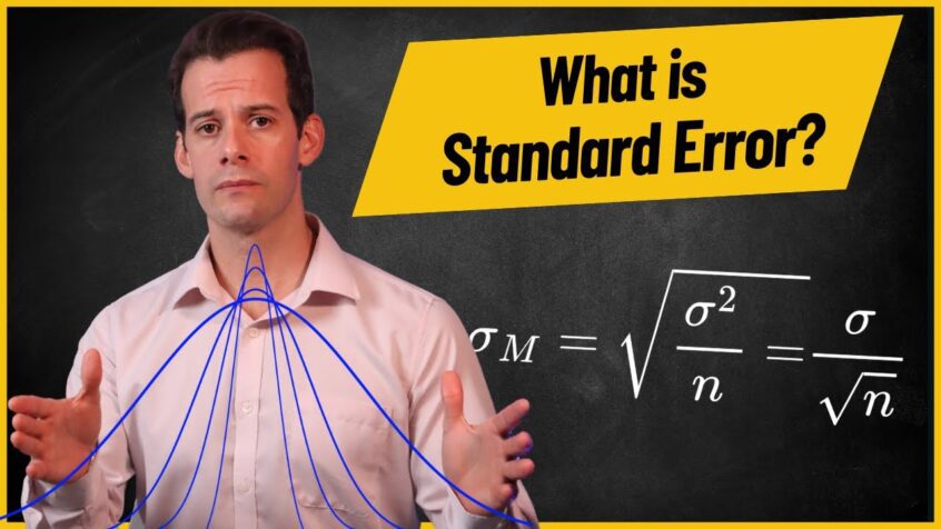
Now variance is, you know, these squared values and so we end up with these numbers that don’t really compare well with our data directly, right? We’re thinking about maybe a population of scores but we look at our variance we say, well, I don’t really know what this means in terms of my score values. And so generally what we do is, we instead use the standard deviation. And the standard deviation is the square root of the variance. And so if we want to know the standard deviation of the sampling distribution of the mean, all we have to do is take the square root of this equation. So the square root of sigma squared is sigma, divided by the square root of n. And so this is the equation for the standard deviation of the sampling distribution of the mean. And you might have noticed it’s very annoying to say “the standard deviation of the sampling distribution of the mean” and so instead we tend to call this the standard error.

So the standard error gives us a sense of how a particular sample mean relates to the population mean, because if we have a really small standard error what that means is the distribution of possible means is really narrow. It’s really tight together and since it’s going to be centered on the population mean that sort of gives us a restricted range of possible values for the population mean. On the other hand, if we have a really large standard error, our means are very spread out for different samples. And so we have less certainty that a particular sample’s mean is actually all that close to the population mean. It might be fairly far away and that might be fairly common if we have a large standard error. And so we can think of this as narrowing our range; giving us a range of values where we think the population mean is going to fall because generally we don’t know the true population mean but we do know that the sampling distribution of the mean is centered on it.

So if we have a small standard error we can say “okay, there’s really good chance the population mean is in this range, and it’s a very small range.” On the other hand, with a large standard error, we have much less certainty. And this is something that we’re going to look at in more detail when we look at the calculation of confidence intervals.

So let’s look at an example of a population distribution and consider what the sampling distribution of means would look like for different sample sizes and what it can tell us about the probability of different samples that we might get, and this will also allow us to review the concept of z-scores.

In this case we’ll use a population where we actually know the population mean so that we can see how different sample sizes would influence the probability of getting a sample mean that’s a particular distance from this known value. So let’s imagine that we’re randomly selecting students and looking at one of their SAT scores out of 800. Now the SAT is a standardized and normed test and so we have a clear sense of what the population should look like. We can expect that the population mean for one section of the SAT will be a score of 500 with a standard deviation of 100 points.

If we randomly selected an individual score from the population with a score of 515 and we wanted to know the probability of selecting a score at least this high, in this case we’re using an individual score. So we could just use the distribution of the population, calculate a z-score for this student, and determine the probability of a single score falling at this point, 515, or greater. So for a single individual a score of 515 from a population with a mean of 500 and a standard deviation of 100 would have a z-score of 515 minus 500 divided by 100 equal 0.15. Then we could look at a z table, we’d find a z-score of 0.15 would have 55.96% of scores below that point with 44.04% of scores falling at or above that point. Therefore when selecting a single score from the population there would be a 44.04% probability of getting a score of 515 or higher; and so this would be a fairly common occurrence.

But what if we were looking at a mean for a sample of scores? In this case we can’t use the population of individual scores and instead we must use the sampling distribution of the mean in order to find the probability. So let’s say that we selected a sample of 36 students and we found that their average score was 515. How likely would it be to get a mean at least this high?

Well first we have to determine the characteristics of the sampling distribution of the mean. The Central Limit Theorem tells us that this distribution will be centered at 500, just like the population, and it will be normally distributed. To find the standard deviation of the distribution of means, or the standard error, we would divide the standard deviation of the population, which is 100, by the square root of the sample size, which is 36. So 100 divided by 6 gives us a standard error of 16.67. Next we can determine the z-score for this point in the distribution of means; 515 minus 500 divided by 16.67 gives us a z-score of 0.899 which we’ll round to 0.9 to look up in a z table.

Now notice that this z-score is higher than the z-score for a single score of 515 because it’s less likely to get an average of 515 for a group of scores. In this case a z-score of 0.9 means that 81.59% of samples would fall below this point and only 18.41% of samples would have an average at this point or above. So the probability of getting a sample of 36 students with an average of 515 or higher would be only 18.41%, much less likely than a single score.

And now we can repeat these calculations for larger sample sizes. If we randomly selected 100 students and we got a mean for our sample of 515 our distribution of means would still be centered at 500 and it would still be normally distributed, but the standard error would be decreased. It would be 100 divided by the square root of 100, or 10. Now a mean of 515 would represent a z-score of 1.5 for this distribution of means. 93.32% of means would fall below this point, meaning that if we took a sample of 100 students the probability of getting a mean of 515 or greater would drop to just 6.68% of samples.

Finally we could greatly increase the sample size to 400. This would decrease the standard error to 100 divided by the square root of 400, or 20, for a standard error of just 5 points. With a sample of 400 students getting a mean of 515 would now have a z-score of 3, and would represent a very unlikely result. 99.87% of samples of 400 would have a mean below this point and only 0.13% of samples of 400 students would be expected to have a mean of 515 or greater by chance alone.

This demonstrates that if we draw a sample of 400 students from the population, we’re very likely to get a mean for that sample that is quite close to the true population mean of 500 and we’re much less likely to get a mean that is farther away. With sample sizes of 400, 68% of sample means would fall between 495 and 505, within one standard error of the population mean, and 95% of sample means would fall within 2 standard errors, or between 490 and 510, and so a result of 515 like ours would be very unlikely to occur by chance.

You should also notice that in order to cut our standard error from 10 down to 5 in the last two examples, we had to quadruple the sample size from 100 to 400. And this is because we’re taking the square root of n. So if we want to increase the denominator by a factor of 2 to cut the standard error in half, this requires increasing the sample size by a factor of 4. And this is useful for thinking about the diminishing returns of increasing sample size to reduce the standard error. At a certain point it may become impractical to continue increasing our sample size in order to get a smaller standard error. If we already have a fairly large sample, it might not be reasonable to try to quadruple that sample size just to cut the error in half.

If we’re reporting the standard error, this is generally done using the abbreviation SE for standard error or SEM for standard error of the mean. And it’s also common to illustrate the standard error by using what are known as “error bars“, which look a bit like capital letter I’s centered over the mean and which span twice the distance of the standard error; extending from one standard error above the mean down to one standard error below the mean. And these indicate the level of uncertainty around that mean based on the standard deviation of the population and the size of the sample. Larger error bars indicate greater uncertainty about how well that mean might represent the population, while smaller error bars indicate lower standard error and therefore less uncertainty.

If there’s one thing that I hope that you get from this video, it’s the fundamental value of being able to calculate a mean. In one of the first videos in this series, I talked about levels of measurement, or types of data. And we looked at nominal, ordinal, interval, and ratio level data. One of the things that I said is if you have nominal or ordinal level data then you can’t calculate a mean for those, it just doesn’t really make sense. And if you can’t calculate a mean, you’re very limited in the analyses that you can do. And hopefully this video has given you a better appreciation for why that is.

Hopefully you see that once you have interval or ratio level data you can calculate a mean, and if you can calculate a mean for your sample then you can think about the distribution of means. And that means that if you have large enough samples you have the central limit theorem to sort of help you out. It says “okay, that’s going to be centered on the population mean.” So even if you don’t know what the population mean is well you have a pretty good way of sort of narrowing it down, and you can think about your standard error and how close you might be. And you can also think about probability because the sampling distribution of the mean is going to be normally distributed, even when your population isn’t. And so you might say, “well, my population is skewed or, you know, it differs from normality in some way, but that’s okay because the sampling distribution of the mean will still be normally distributed and I can use that to estimate some probabilities.” And so all of this is what makes the mean such a powerful statistic. And hopefully if there’s one thing you get from this video, it’s that understanding of the importance of the mean for so many different statistical analyses.

Okay, so that is the sampling distribution of the mean, the central limit theorem, and the concept of standard error. I hope that you found this helpful! Let me know in the comments if you did, feel free to ask other questions that you have and I’ll try my best to answer them, and be sure to like and subscribe and check out the hundreds of other psychology and statistics tutorials that I have on the channel.

Thanks for watching!