In this video I describe box-and-whisker plots, or boxplots, developed by John Tukey. First we’ll look at a simple box-and-whisker plot, then we’ll see some variations depending on the data, some different sets of terminology that can be used when creating boxplots, and how we can use boxplots to get a quick visual sense of differences between distributions.
For more detail on different methods for defining hinges or quartiles based on sample size, I recommend checking out the explanations in the following links: https://peltiertech.com/comparison/ https://peltiertech.com/quartiles-for… https://peltiertech.com/quartiles/ https://peltiertech.com/hinges/ https://www.statisticshowto.com/upper-hinge-lower-hinge/
Video Transcript
Hi, I’m Michael Corayer and this is Psych Exam Review. In this video we’re going to look at another form of exploratory data analysis, also developed by John Tukey, which is the box and whisker plot or box plot. This is a common way of visualizing a set of scores in order to get a sense of the distribution. So we’ll start by seeing how we create a box and whisker plot then we’ll talk about some variations that may occur in the plot depending on the data that we have. We’ll also look at some slight differences in terminology that are used depending on how we define particular parts of the box plot, and finally we’ll see the usefulness of boxplots when it comes to comparing multiple sets of scores.
So here we have a set of scores and in order to create a box and whisker plot for this set of scores we need to know five key values. These are the maximum, the minimum, the median, and then what Tukey called the hinges; the lower hinge and an upper hinge. So we can start with the maximum, which is our highest score, which is here at 92. Then we have a minimum of 54. and to find the median we have an odd number of scores so it’s going to be in the middle position, here the seventh position in a set of 13 scores, and that’s 82.
And now we need to find these hinges, and these are essentially the median of the lower half of the data and the median of the upper half of the data. And so in this case we’re going to use an inclusive median; we’re going to include 82 as part of the lower half of the data and we’re going to include it again as part of the upper half of the data. And if we do this then we see the middle point here is at 70. We have three scores then 70 and then we have three scores up to and including the median of 82. And then we can do the same process or the upper half of the data and that will give us an upper hinge of 88.
So in order to understand this process of finding the hinges, Tukey thought of it as a folding process; we’re deciding how we can fold the data up into four sections and to see that we can have a visual presentation of the data.
So here we can see we’ve folded the data up into four sections. We have the median at 82 and then we have these folding points, or these hinges, in the lower and upper halves of the data and those are falling at 70 and 88.
So now that we have our five key values we can start plotting our box and whisker plot. In this case I’m going to plot it vertically but you could plot it horizontally if you prefer. So we start with our median value which is 82, and we’re going to draw a line here at 82. And then we have our upper hinge which was at 88. And we have our lower hinge down at 70. We have our maximum at 92. And we have a minimum down at 54.
So now we’re going to connect the hinges in order to create a box in the middle. And once we’ve created this box now we can add in the lines for the whiskers. Ok, so now we have our box and whisker plot and the question is, what does this tell us about the distribution? What should we look for when we look at a box and whisker plot? So the first thing that we should look at is the location of the median. So that’s this line in the middle of the box and what this is telling us is about the spread of the scores from the median up to the upper hinge and down to the lower hinge.
Now remember that the number of scores between the median and the hinges, the upper hinge and the lower hinge, is going to be the same. The location of the line is telling us how spread out those are. So if the median is closer to the upper hinge then those scores are less spread out and if it’s farther from the upper hinge then that tells us that the scores from the median to the upper hinge are more spread out, and from the median down to the lower hinge are less spread out. We can also look at the distance from the upper hinge to the lower hinge.
So in this case we have a distance from 88 down to 70, and that distance is 18, and this is what Tukey called the hinge spread or the h-spread. That’s telling us the spread of approximately the middle fifty percent of our set of scores. And then we can look at the whiskers. So the whiskers are telling us about the distribution from the upper hinge to the maximum and from the lower hinge down to the minimum. Now again if the whiskers are symmetrical that tells us that the spread of those scores is roughly equal, but if they’re asymmetrical, as they are in this case, that’s telling us that this same number of scores from the upper hinge to the maximum is much less spread out than that same number of scores from the lower hinge down to the minimum. So in this case we have much more spread in our scores going down from the lower hinge down to the minimum.
And we can also see the overall range of the entire set of data. So the range would be the distance from the minimum to the maximum. And so in that case we would have 92 minus 54 equals 38. So by looking at a box plot, looking at the symmetry of the median in relation to the box, and looking at the symmetry of the whiskers and the overall distance of the h-spread compared to the range, we can get a sense of how the scores are distributed in different parts of the set of scores. So that’s how a simple box and whisker plot works and now we’re going to look at a second set of scores where we have some minor adjustments that we’re going to make to how we draw the whiskers and how we include outliers in our data.
So here we have a set of 14 scores and in this case as we find our five key values we’re going to see that there’s some things about this distribution that are going to cause us to slightly change some of the things that we put into our box and whisker plot. So if we look at our maximum value we have 90, and then we have a minimum value of 0, which is very low, and next we need to find our median. And in this case we have an even number of scores so it’s going to be the average of the middle two values, so our median will be here at 75.5
Now in this case we’re going to use an exclusive median, we’re not going to include 75.5 as part of the upper and lower halves of the date, so if we look at this lower half then we have a hinge here and if we have the upper half here starting with 76 then the upper hinge will be here at 82. We have 82 for our upper hinge and 66 for our lower hinge. Now when we look at this distribution we see that we do have some extremely low scores and we might not want to extend the whiskers of our box and whisker plot all the way to these maximum and minimum values because they’re very spread out. And so in this case we’re going to see that maybe we have some outliers. So we’re going to define what we consider to be an outlier and then that’s going to change how we draw our box and whisker plot.
So we can start by looking at the hinges. So we have this h-spread in this case that goes from 82 to 66, and so that’s going to give us an h-spread of 16. Now we have these values that are very far below that hinge spread and so we’re going to do is we’re going to define these as outliers, and the way that we’re going to do that is we’re going to use this h-spread times 1.5 and this is going to set our fences, so if we do that then we get a value of 24. And we’re going to say that if a score falls more than one and a half times the h-spread below the lower hinge that we’re going to consider that to be an outlier and we would do the same for the upper hinge. If a score is more than 24 above the upper hinge then we consider that to be an outlier. And so we’re going to set what we call fences for what we consider to be outliers versus the rest of our data and so our fences are going to be the lower hinge minus 1.5 times the h-spread, which is 24, and that means that we’re going to set a lower fence of 42.
And we’d set an upper fence of 82 plus our 1.5 times the h-spread and that’s going to give us 106. So if we had values that are below 42 then we’re going to consider those to be outliers, and if we have values that are above 106 we would consider that to be an outlier. And if we look at our data then we can see that we have some outliers here, right? We have scores that fall outside of these fences and so now when we draw our box and whisker plot instead of extending our whiskers all the way to the maximum and minimum of the entire set of data, we’re just going to draw it to the nearest values that are within those fences. So let’s look at how we would draw this.
We’ll start plotting this just as we did before, by starting with the median which is at 75.5 and then we’re going to put in our upper hinge which is at 82. And we have a lower hinge at 66. And now instead of using the maximum and minimum values we’re going to use the maximum or minimum that are still within our fences. So what scores are closest to 1.5 times the h-spread subtracted from the lower hinge or added to the upper hinge? What are the values that are closest to that? What are the adjacent values to those points? And in our case if we go to the maximum. Well it’s still within the fence, so 90 is beneath 106, so in that case we’re still going to draw our maximum at our actual maximum for the distribution. But our minimum if we use the fence is actually 45. That’s the closest score that we have without going beyond the fence. So now we’re going to draw our minimum for our whisker at 45.
And now we can add the fact that we did actually have scores beyond this point. So this box of whisker plot is telling us where most of our data was, but with the idea that we had some outliers. We have an outlier at 38, that’s beyond our fence, so we’re going to draw that in here with a circle. And then we actually had another outlier all the way down at 0. And in this case it’s actually more than 3 times the h-spread subtracted from the lower hinge. And so that will be defined in Tukey’s terms as being “far out“. Not just outside the fences, but far out, or what we also might call an extreme outlier. And so that’s all the way down here at 0. Now in some cases you may indicate far out scores a little differently than outliers. Sometimes they’ll be shown exactly the same, just as a circle, Tukey sometimes did this by putting a circle around a dot to indicate an extreme outlier. You may also see it drawn as an asterisk to indicate that it’s an extreme outlier. Or you may just see it as a dot just like any other outlier.
So a common question that students have about whiskers in this situation is why we extend them to the adjacent value rather than to the fences that we’ve created. The reason for this is that if we extend them to the fences then they’ll always be symmetrical, because the fences will be symmetrical. But now we’re getting less information about the distribution, right? We want to see if the whiskers are asymmetrical. Where do the values actually extend to? And setting the whiskers to end at the adjacent value helps us to see that. We can see if we have values close to the fence above the upper hinge or close to the fence below the lower hinge and we can also see if we have outliers. So if we have scores beyond those fences then those will be indicated as outliers, and so we’ll know that we had scores there.
And so that’s why we extend to the adjacent value rather than just extending it symmetrically to the fences. So now we can see what we learned from looking at this box plot. We have our median here which is fairly symmetrical, so the same distance roughly from the median up to the upper hinge and down to the lower hinge, and as we saw before we had an h-spread here of 60. Then we have the range of our data that is not considered to be an outlier, so that range would be from 90 down to 45 and so our range there would be 45. And then we can also see that we have outliers; we have one outlier here and then we have this other outlier all the way down here.
So in the case that we have outliers in our data then it’s going to slightly change how we set the whiskers but the same things that we observed before still apply. We can look at the length of the box, where the median is positioned within that box, and whether the whiskers are symmetrical or whether they’re asymmetrical and how spread out different sections of our data are. So here we have the same set of data put into a software program in order to generate a box and whisker plot and this brings up some minor differences in terminology. So in this case the software isn’t actually finding “hinges”, it’s finding Q1 and Q3, and these are the 25th and 75th percentile.
And these might be slightly different from the hinges. It depends on the data that you have. If we look at our very first set of scores and you put those into a spreadsheet and you calculate these values you’ll find they’re actually the same as the hinges but in the second set of data you’ll find that they differ slightly. That’s because when we’re using hinges we’re finding the values in our set of scores that are closest to the 25th and 75th percentiles, but the software program is finding the precise values of the 25th and 75th percentiles. And so if we put this set of scores into a software program it’s going to tell us that Q1 is not the hinge of 66 that we had, it’s actually 66.5 and Q3 is not the hinge of 82 that we had, it’s actually 81.75.
Ok, so they’re going to be slightly different and this is also going to depend on whether we are using an inclusive or an exclusive median, and it’s going to depend on whether it’s interpolating values which means that it’s finding values between your scores rather than just using scores, and it’s also going to depend on whether we have multiple scores that are sort of stacked up at certain points. So if you have repeated scores at different points in your data that can also influence these calculations.
Ok, so since we’re no longer talking about hinges we’re also not going to talk about the hinge spread or the h-spread. Instead we’re going to talk about the distance between these quartiles and so we’re going to have the interquartile range. Again it’s essentially the same as the hinge spread, it’s the same concept, it’s just calculated more precisely. And so in our case we had an h-spread of 16 but if we use these new values for Q1 and Q3 that are slightly different then we’ll find that it’s going to give us an interquartile range of 15.25.
But otherwise we can see that this doesn’t really have a major effect on the appearance of the boxplot, right? It’s still telling us essentially the same story. We can see the location of the median compared to Q1 and Q3 and whether this is symmetrical or whether the scores are distributed slightly differently. We can also look at the length of the whiskers to see how the scores are distributed beyond those points, and we can also see that we had some outliers indicated and so we have scores that are going to go beyond our fences, right? They’re more than, in this case, 1.5 times the interquartile range below Q1 or in this case with the extreme outlier, more than 3 times the interquartile range past the Q1 point. And again you’ll notice that this is created in R studio and it doesn’t specify that this is an extreme outlier, right? It just uses a circle for any outliers.
But just by looking at this we can tell this is an extreme outlier, because we can see roughly the distance of the interquartile range. We can see where Q1 is here and we can see that this distance is going to be more than three times this distance of the interquartile range and that means it’s going to be an extreme outlier.
Ok, so now we’ve seen some different variations on exactly how we draw a box plot depending on the data that we have, and hopefully we’ve clarified any confusion about some different sets of terminology that you might see. Now if you are still getting a bit stuck on some of the terminology remember that that’s not really the most important point. What we want to get is what we can learn from looking at a box plot. What is this telling us about the distribution of our scores?
In exploratory data analysis we’re doing what Tukey called “detective work” so we’re just looking for what clues are there here that might be interesting about this distribution of scores? That’s much more important than thinking about you know was this an inclusive or exclusive median? Is this a 25th percentile or is it a hinge, you know? Those small differences do matter in some sense but they’re not the most important thing when you’re looking at a box plot. What you want to be thinking about is “what is this telling me about the distribution of scores?”.
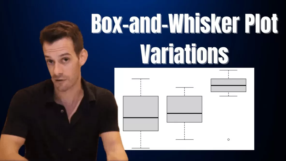
And this brings us to one of the most important uses of the box plot, which is that we can use it to compare multiple sets of scores all in the same image. So now we can take what we’ve learned about looking at a single box plot and what we should be looking for and we can apply it to looking at multiple box plots in the same image. So here we have three different groups that have been assessed for some variable and we’ve created box plots of their distributions and we can see that there’s some differences between these groups.
So we can look at the length of the box, that’s telling us the middle fifty percent of the scores right? The interquartile range or the h-spread if we were using hinges, and we can see that, you know, groups 1 and 2 are fairly similar, you know? Group one is a little bit more spread out but group 3 is very different; it’s a very narrow interquartile range. Here these scores are really closely clustered together. And we can also look at the position of the median in comparison. We see in group three it’s pretty much perfectly symmetrical, not so in the other two groups. Although, you know, maybe it’s not large enough of a difference for us to really be concerned with and we can also think about how the whiskers differ.
So we can see in group 1 the whiskers are fairly symmetrical and they’re pretty spread out from the 75th percentile and the 25th percentile. In group two we have a little bit less spread of the whiskers and they’re a little bit asymmetrical. This bottom whisker is a little bit longer than the top whisker, so the scores are a little bit more spread out from the minimum value up to Q1, or the 25th percentile, than they are from the 75th percentile up to the maximum. And in group 3 we can see they’re much more narrow. So this whisker is very short, extending down in this case to whatever value is closest to the fence that we have, and the maximum value here extending up a little bit longer. And we can also see that we have an outlier down here. So we have one extreme score that’s quite different from the rest of the scores in this group and so we might want to think about what that might means, what that might indicate.
We could also notice something that, you know, this score is an extreme value in comparison to the rest of scores in group 3, but if this score were in group 1, well it wouldn’t be an outlier, right? These scores are much more spread out and so it wouldn’t be an outlier if it were in this set of data. But when we’re comparing it to the rest of the scores in group 3 it’s very different, right? So we could think about what might this be indicating about these groups. Group 3 seems to be quite different from groups 1 and 2. So this shows us the usefulness of box and whisker plots for comparing different sets of scores because we can look at this and immediately see differences in the distributions. We can look and say group 3 seems to be distributed quite differently compared to groups 1 and 2.
Now it doesn’t tell us the exact magnitude of these differences in terms of statistical analyses, and it certainly can’t tell us why group 3 differs from group 1 and 2, but it tells us that there’s a clue here, right? Remember in exploratory data analysis we’re doing this “detective work”, we’re looking for clues about the distribution. We’re trying to get a sense of it and so this image can give us a very quick sense of differences between the distributions, compared to doing something like looking at a table with a bunch of numbers that would be much harder to see these differences.
And so that’s why box and whisker plots can be very useful when it comes to comparing multiple sets of scores. Ok, so that’s box of whisker plots, I hope you found this helpful. If so, like and subscribe for more educational content on psychology and statistics, let me know if you still have questions in the comments and I’ll try my best to answer them, and make sure to check out the hundreds of other psychology tutorials that I have on the channel. Thanks for watching!