In this video I explain how to use the interquartile range in order to identify possible outliers in a data set. This can be done using the interquartile range times 1.5 for moderate outliers, or times 3 for extreme outliers. This distance then creates a boundary below the 25th percentile and a boundary above the 75th percentile, creating a range for acceptable data points and excluding scores below and above those boundaries from analyses.
Video Transcript
Hi, I’m Michael Corayer and this is Psych Exam Review. In addition to using the interquartile range to understand the spread of data around the median we can also use it to define outliers in our data and then potentially remove them before we do other analyses.
Now before we start thinking about identifying outliers and removing them, we always want to think when we see extreme scores: what are the possible causes of this? And one possible cause is always input error. Maybe you were just copying the data into a spreadsheet and you hit an extra key or you made a mistake and this means it’s not a genuine score. It’s not an outlier it’s a mistake.
Or it could be the case that it was a measurement error. While you were recording reaction time a participant sneezed on one of the trials and so now again it’s not an outlier that they had extremely slow reaction time, it’s that there was an error. Or it could be the case that a participant misunderstood the instructions, so they weren’t doing the task correctly. In this case we might decide that we need to remove all of that participant’s data because they didn’t just misunderstand the instructions this one time and got an extreme score, maybe on the other scores that weren’t so extreme they also weren’t doing things right. They weren’t, they weren’t doing the task that you thought you were measuring.
And it could be the case that the participant is not appropriate for the sample that you have and that’s why they’re so different from all your other participants. And so in this case you might want to think about your sample and how representative it is for the population that you’re trying to investigate. So we have to consider all of these options, not just how extreme a score is before we decide whether or not to remove it.
But if we think we have a genuine measurement, so it’s really measuring what we thought we were measuring and it represents a true response from a participant, but it’s extremely low or extremely high, now we have to think about what to do about this. Now on the one hand we can say “well, we keep it in because that makes the data more accurate”. On the other hand we can say “well, it might be more accurate but this extremely high or low score is actually going to have a misleading effect on some of the analyses, so now they might not really represent the rest of the sample and maybe not the rest of the population. And so these analyzes will end up being misleading if we include these outliers.” Here again we see this key theme of statistics, which is researchers have to make choices and the choices that they make are going to influence the results and how the data is presented.
Now in the case that we remove outliers we don’t simply delete them and pretend they were never there. We have to explain why these were removed. We have to give a justification. This is where the interquartile range comes in because it gives us a possible mathematical justification for why we want to exclude certain data from certain analyses. So how do we use the interquartile range in order to define outliers?
Well, we start by finding the interquartile range then we take this value and we multiply it times 1.5 and then we take this new value 1.5 times the interquartile range and we subtract it from the 25th percentile. This is going to give us a lower boundary. What we’re going to say is anything below that point, anything below 1.5 times the interquartile range subtracted from the 25th percentile, anything below that is going to be considered to be a moderate outlier. And then we do the same at the 75th percentile: we take 1.5 times the interquartile range and we add it to the 75th percentile and then we say anything above that is a moderate outlier on the high end.
And so now we have these two boundaries sort of fencing in our data that we’re going to consider acceptable for our analyses, and anything more extreme than that is going to be considered an outlier. Now we can also do this for what we call extreme outliers and this is the same idea but in this case we’re going to multiply the interquartile range times 3. So now we’ll have a much lower boundary on the lower end and a much higher boundary on the upper end. So we’ll include more data in this case and we’ll eliminate fewer outliers, only the most extreme ones.
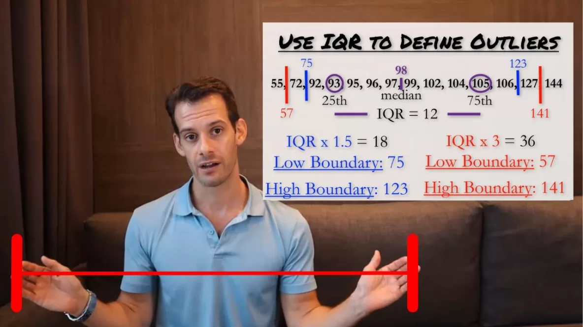
So let’s see what these calculations would look like with a set of scores. In this case we have 14 scores, so our median is going to be the mean of the 7th and 8th positions. So that gives us a median of 98. Now we find the 25th percentile which is 93 and the 75th percentile which is 105. Now to find our interquartile range we take 105 minus 93 and we get 12. Now we multiply 12 times 1.5 this gives us 18. So we take 18 and we subtract it from the 25th percentile so we get 93 minus 18 gives us 75. So that sets a lower boundary. It says anything lower than 75 is an outlier. Then we take 18 and we add it to the 75th percentile which is 105. So that gives us 123. So we say anything higher than 123 is an outlier. So as we can see this would remove 4 scores from our data. We have 2 scores below our lower boundary and 2 scores above our upper boundary.
Now if we thought that this was being too stringent and too narrow with what we defined to be our acceptable data, then we could use interquartile range times 3. So this would only remove extreme outliers and so we would take 12 times 3 is 36 so then we’d subtract 36 from our 25th percentile so we get 93 minus 36 is 57. And then we would add it to our 75th percentile so we’d have 105 plus 36 is 141. So now we’d say that any scores below 57 would be outliers and any scores above 141 would be outliers. So this gives us a broader range for our data and only eliminates the most extreme of outliers.
Now of course I want you to keep in mind that this is a very small sample and I’ve intentionally chosen these values in order to have outliers to remove. Now it looks like, wow, this is really getting rid of a lot of data here. But if you had data for something that approximates a normal distribution and you had a large set of data then you’d expect that using interquartile range times 1.5 should only remove about 0.7 percent of your data and if you’re using interquartile range times 3 then this should only remove .002 percent of your data, or about one in fifty thousand scores. And so I think there you’d see that it’s more justified to say this really is an extreme value. This is a score that happens, you know, once in every 50 000 scores. Maybe we’re justified in setting it aside while we do our analyses.
This is not the only way to define outliers and once we’ve gone into a bit more detail on normal distributions, standard deviation, and z-scores, we’ll see another approach. I hope you found this helpful, if so, let me know in the comments, make sure to like and subscribe, and check out the hundreds of other psychology tutorials that I have on the channel. Thanks for watching!