
In this video I describe the 4 scales of measurement proposed by Stanley Smith Stevens, which have become the standard way of defining types of data. These include nominal, ordinal, interval, and ratio. I discuss the defining features of each, provide a few examples in psychological research, and mention the descriptive statistics that can be applied for each type. I also explain the distinction between continuous and discrete variables that can be used when discussing interval or ratio data.
You can find the original 1946 paper by Stevens here.
Below are the summary slides for each data type, if you’d like to download these click here.
Video Transcript:
Hi, I’m Michael Corayer and this is Psych Exam Review. In this video we’re going to look at the four scales of measurement proposed by Stanley Smith Stevens in a paper in Science in 1946, and this was to clarify some confusion over different types of data. At the time sometimes data was referred to as intensive data or extensive data and Stevens wanted to clarify and so he provided four ways we can classify our types of data. You may also see this called levels of measurement or just types of data, and I’ll post a link in the video description where you can find the original paper if you’d like to take a look.
So these are now generally accepted as the ways that we can classify data and the reason that this is important is because it tells us what kinds of statistical analyzes we can do with the data. So we have to know what type of data we have in order to determine what type of tests and what types of calculations we can do with that data. Now in this video we’ll look at these four types, I’ll give a few examples of each, and I’ll talk about some of the statistics that can be used based on each type of data. And what you’ll see is that this is cumulative; with each new type that we look at it will be able to do the calculations from the previous type as well as some new additions. So these four scales that Stevens proposed are nominal, ordinal, interval, and ratio, and you can remember these with the mnemonic NOIR.
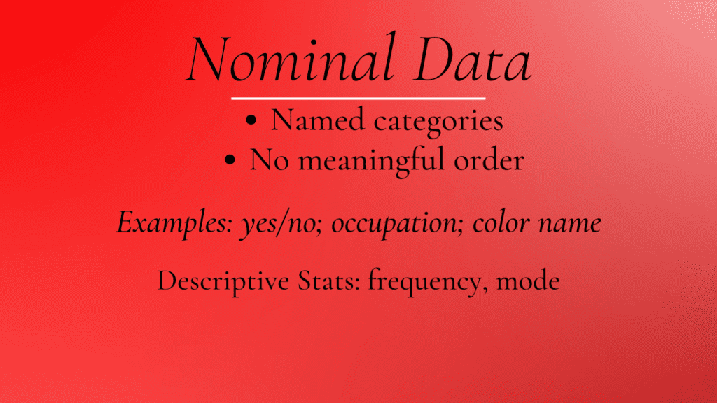
So first we have nominal data and this comes from the Latin “nomen” for name and it means we just have named categories. So participants give their response and it falls into one of the categories that we’ve created. And an important point about these categories is that they can’t really be compared to each other, so there’s no meaningful way to order arrange or rank them. So a very simple type of nominal data would be a yes no response. So we have these binary categories, participants can either fall into yes or no.
But we could have many other categories. We could do something like an occupation. So participants would select which category best describes their occupation but we wouldn’t really have a way to compare those responses. Or if I ask people their favorite color; so if half my participants say red and half say blue now you see that I can’t really do something like find the mean. I can’t take the average color that people like. I can’t find a median, I can’t line these scores up and see what’s in the middle. So all I can really do with nominal data is talk about the frequency of the different responses. I can say this percentage of participants fell into this category, this percentage fell into this category, etc. And the only central tendency that I can find would be the mode that would be to talk about the most common response in the data. Here’s a slide summarizing nominal data and if you’d like to copy of these slides I’ll post a link in the video description where you can find them.
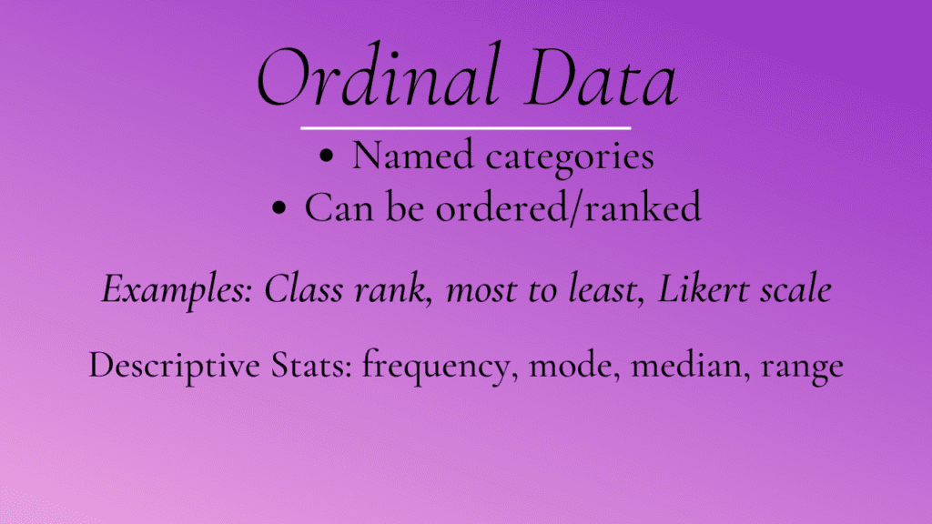
Now if we can put our data into an ordered set of categories then we move to the next scale of measurement and that would be ordinal data. In ordinal data we’re still talking about named categories but in this case we can put them into a meaningful arrangement, we can order or rank them. A simple way to think about this is runners in a race. We can say this person came in first, this person came in second, this person came in third, etc. But what we see is that the distances between those are not necessarily equal. So the distance between coming in first and second might be very different from the distance between second and third and this means that we can’t do things like find the mean.
Another way to think about ordinal data would be if I had a room full of people and I decided to rate them from least attractive to most attractive. So this would allow me to put them into a meaningful order but if you just knew that somebody was fifth it wouldn’t tell you very much because you don’t know how far away they are from first or last, and so you don’t really know that much about how attractive they are.
Now a common type of ordinal data in psychological research is the use of a Likert scale. This is named after Rensis Likert, and you’ve probably seen one of these if you’ve done a survey before. So you might have a statement and then you can be neutral, you can agree, or disagree, or you can strongly agree, or strongly disagree. And there could be a different number of options but usually it’s about five. What we see now is we can put all the responses in order, but it’s not really clear what this order means because we don’t know that the distance from agree to strongly agree is the same as the distance from disagree to neutral. So we can’t really tell very much. We can’t calculate a mean. So if half my participants strongly disagree and half of them strongly agree it doesn’t really make sense to say that on average they were neutral, that doesn’t really work. But what we can do is we can put the responses in order and that means that now we can find a median and we can also talk about a range. So we can say this was the lowest response and this was the highest response and that gives us a range of all the data. So here’s a summary of ordinal data and what we’ll see in the next type is if we do have equal distances between these points now we move to what’s called interval data.
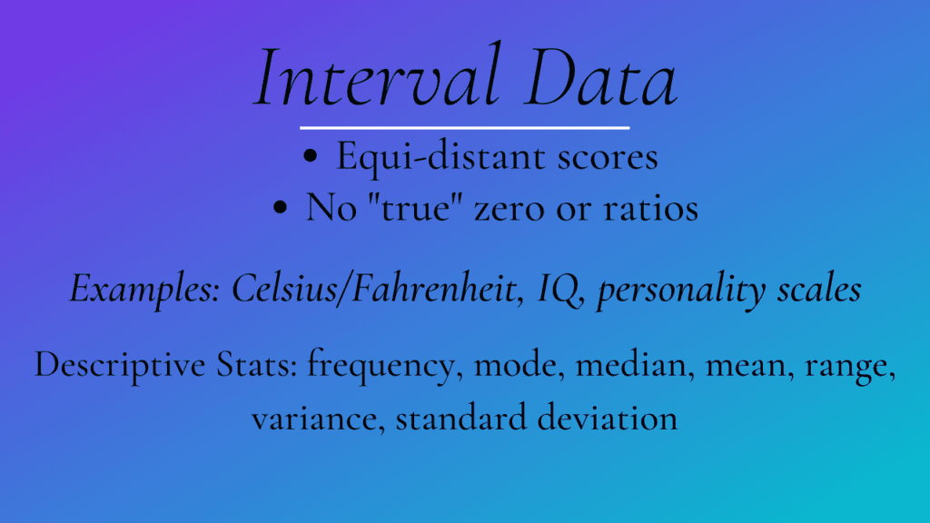
Now, rather than just categories we can start talking about responses as scores. So we have an order to the responses and the distances between all the possible responses are equal. A textbook example of interval data is temperature in Celsius or in Fahrenheit. So the distance between each degree in these scales is the same; going from 20 degrees Fahrenheit to 21 degrees Fahrenheit is the same as going from 85 to 86. Now the problem we have with interval data is that we don’t have a true zero.
So what a true zero means is that there’s no measurement and so in the case of temperature when we say it’s zero degrees Celsius we don’t mean that there’s no temperature or there’s no heat. It’s not a true zero; it’s an arbitrary point, or as Stevens wrote the zero in an interval scale is “by convention or convenience”. In the case of Celsius we chose it based on when water freezes but we could have chosen any other point, it doesn’t really matter.
Now because we don’t have a true zero this also means that we can’t really talk about ratios. So you could think about this with temperature. If we said that it’s 20 degrees that doesn’t mean that it’s twice as hot as 10 degrees. Or we could return to our running example. We can apply interval data there instead of just saying first, second, third. What we could do is measure the time after the winner; so we could say the person in the second was 10 seconds behind the winner and the person in the third was 30 seconds behind the winner. That would be interval data. The problem that we’d have is it’s an arbitrary zero, so what that would mean is we couldn’t say that because the person in third was 30 seconds behind and the person in second was 10 seconds behind, that the person second was three times faster. It just doesn’t work that way because it’s an arbitrary zero. We need to know how long it took the winner to run the race in order to start making those kind of ratios.
Now for a psychological example of interval data we could think about something like IQ score. So this is an interval scale because each point on the IQ scale is considered to be the same distance; from 83 to 84 is the same as from 102 to 103. But we can’t use ratios. We don’t say that someone with an IQ of 120 is twice as smart as somebody with an IQ of 60. And we don’t have an idea of a meaningful zero when we talk about IQ score. We can’t say that there was no intelligence measured at all and this would also apply to other assessments in psychology for things like personality traits. We don’t have an idea of a zero agreeableness or extraversion and we can’t really talk about those scores as being twice as agreeable as somebody else. But the fact that we have even spaces in interval data means that now we are allowed to calculate a mean or an average, and this also allows us to calculate things like variance and standard deviation. So here’s our summary of interval data and this brings us now to the last type, the last scale of measurement, which is ratio data.
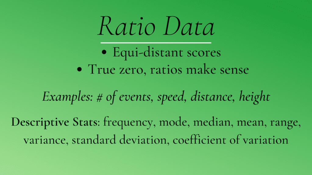
Ratio data has all the features of interval data but it also has the idea of a true zero and that means that we can calculate ratios. So if I measure your time for an entire race now I can start saying, you know, this runner was twice as fast as this other runner. You know, they ran the race in four minutes and the other person ran the race in eight minutes so now those ratios make sense because we have a true zero, which would be you know at the very start of the race, everybody’s starting from the same point, that same zero measurement. The same would be true if I were to measure something like the speed of a car. So at zero there’s no speed at all, the car is not moving. That’s a true zero. And then if it’s going 50 miles an hour I can say that’s twice as fast as 25 miles per hour.
Now for a psychological variable we could think about measuring something like the number of stressful life events that you’ve experienced. So it’s possible to actually score a zero; there’s no measurement there if you haven’t had any stressful life events. And if somebody has had four stressful life events and you’ve had two then we can say they had twice as many as you did. Another way that I could measure is your time to complete a task. So if you read a paragraph in 30 seconds and somebody else read it in 15, you could say they were twice as fast as you.
And this brings up one final distinction when we talk about interval or ratio data and this is the difference between continuous variables and discrete variables. What this does is it answers the question; can the variable take any value or can it only take whole numbers? So in the case of stressful life events that would be a discrete value because you can’t have 3.4 stressful life events. You either have three or you have four. But if I’m measuring something like your time to read a paragraph, then it can take any value. I could say it took you 14.3417 seconds. Now I might not always measure to that level of accuracy, but it’s possible. The underlying variable is continuous. The idea that I’m measuring time in seconds means it could take any value within that. Whereas for other things that you count, like if I ask how many times have you gone to the gym this month, you can’t tell me that you went 12.3 times or you know 14.8 times. You have to pick a whole value; that’s what makes that a discrete variable.
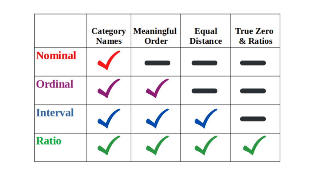
So with ratio data we can do everything that we could do with interval data and we can also calculate what’s called a coefficient of variation, which I’ll talk about in a future video. So here’s a chart that summarizes all the defining features of these four scales of measurement: nominal, ordinal, interval, and ratio. And while these may seem simple and clear-cut, in a future video I’m going to discuss some of the debate that occurs in psychology and other social sciences when it comes to theory versus actual practice.
I hope you found this helpful, if so, please like the video and subscribe to the channel for more. Thanks for watching!