In this video I explain one way in which a distribution can deviate from normality, which is skewness. I explain the difference between positive and negative skew, and how these can be seen in histograms, stem and leaf displays, and box and whisker plots. I then discuss the effect of skew on measures of central tendency and consider possible reasons a sample may be skewed and when we can expect a population to be skewed.

For detail on distributions which violate the general mean-median pattern see von Hippel (2005): https://www.tandfonline.com/doi/full/10.1080/10691898.2005.11910556

Video Transcript

Hi I’m Michael Corayer and this is Psych Exam Review. In the video on histograms and frequency polygons I mentioned how these can be used to help us get a sense of whether our sample is similar to a known distribution such as a normal distribution. This is a symmetrical bell-shaped curve and it’s commonly assumed that many variables are normally distributed in the population.

In this video we’ll look at one way that we might differ from normality and this is in terms of symmetry. So a bell curve is perfectly symmetrical but our sample or our population’s distribution may not be and this asymmetry is referred to as skew.

If we start by thinking of a perfectly symmetrical normal distribution then we’ll realize it could be skewed in either direction; there could be an asymmetry where there’s more scores on the left and then a tail extending to the right or there could be more scores on the right in a tail extending to the left. If we have more scores on the right and the long tail extends to the left then we say that this distribution is left skewed or negatively skewed and if we have more scores on the left and the tail extends to the right then we say it’s right skewed or positively skewed.

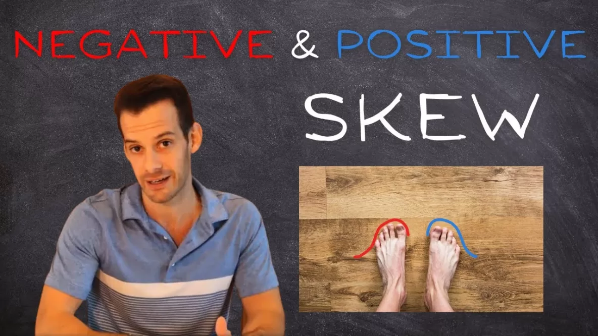
An easy mnemonic to remember this is to simply look down at your feet because your left foot will resemble the shape of a left skewed distribution or a negatively skewed distribution and the shape of your right foot will resemble a right skewed distribution or a positively skewed distribution. And then to remember which is negative and which is positive you can simply remember the phrase having “two left feet” being a negative assessment of your dancing ability. So that will hopefully remind you that the left is the negative skew and therefore the right foot would be the positive skew.

So your feet can represent how you’d see skew in a histogram and the same thing would apply to a stem and leaf display, just oriented sideways. But we can also see skew in a box and whisker plot and we can see this in two ways. We can look at the location of the median within the box, which is the distance between the lower and upper hinge, or q1 and Q3, and we can see that if the median is exactly in the center then it’s symmetrical in that middle part of the distribution. But if the median is closer to the upper hinge or to Q3 then this implies that we have negative skew and if the median is closer to q1 or the lower hinge then this will imply that we have positive skew. And this can also be seen in the length of the upper and lower whiskers. If the upper whisker is longer then that suggests that we have positive skew and if the lower whisker is longer then that indicates negative skew.

In a normal distribution the three measures of central tendency; the mean the median and the mode, will all be at exactly the same point. But if we have an asymmetrical distribution or we have skew then they’re going to become separated, and this is because they differ in their sensitivity to extreme scores.

So if we have a continuous variable and we have a unimodal distribution, meaning we only have one mode, then what we’ll see is the mode will still be at the peak of the curve, so that’s the point where we have the highest frequency, the median will be at whatever point is the 50 point of the data, so the middle value with 50% of scores to the left and 50% of scores to the right. But the mean is sensitive to extreme values so if we have skew and we have some extreme values on one side the mean is going to get pulled in that direction.

And so if we have a left skewed distribution or a negatively skewed distribution what’s going to happen is those extreme values to the left are going to pull the mean to the left. They’re going to pull it downward to be a lower value relative to the median. Then if we have right skew or positive skew then what’s going to happen is the mean is going to get pulled upward. It’s going to get pulled in the positive direction or it’s going to be pulled to the right relative to the median.

Now it’s important to note that this is a general pattern but it’s not a hard and fast rule. So there are some exceptions to this. There are distributions where this won’t be the case. And this can depend on how heavy the different sides of the distribution are, so if you have a really heavy section where most of the scores are and the tail extending off the the skew is very thin, meaning there’s not very many scores there, then that can influence this and it can also depend on if you have a discrete variable or a continuous variable. So when you have a discrete variable then you may see situations where you end up with a mean that’s actually to the left of the median even though there’s right skew. But these are exceptions to this general pattern and if you want to read more about these exceptions then I’ll post a link in the video description where you can read a paper by von Hippel discussing some of these different exceptions to this general pattern. But for the most part if we have a continuous variable and we have a unimodal distribution then we can assume that if we have left skew the mean is going to get pulled to the left of the median and if we have right skew it’s going to get pulled to the right of the median.

So what causes skew? Let’s say that we have a sample and it’s skewed and we want to know why this might be. Well, there’s a number of different explanations. One possibility is that it was just chance. It could be the case that the population is normally distributed but we just happened to select a sample that is, because not every sample that you draw from a population is going to match that population’s distribution. So we could have a normally distributed population and we just happen to draw a sample that is skewed, and this is more likely to be the case if we have a smaller sample size.

But it could be the case that the population is also skewed. So we have a skewed population, we’ve selected a sample from that population that’s also skewed, and that skew is accurately representing the distribution of the population. And so now we’ll look at a few cases where we can expect to see some skew in the population, positive or negative.

Positive skew or right skew will tend to occur in populations for variables where we have a hard lower limit that scores can’t fall below and then we have most scores in sort of the lower part of this distribution. But the upper scores are somewhat unlimited, they can extend very far beyond the point where you’d find most of the scores. And so this results in a very long tail to the right. So you could think of income as a good example of this. Nobody earns less than zero dollars per year and so we have a hard limit on the lower end, and then most scores are going to be above that but then as we extend further away of course the scores become less and less frequent. But they can extend very very far beyond where most of the other values are. So you can have somebody earning hundreds of millions of dollars in a year whereas most people of course are not earning anywhere close to that. And so the result of that is this very long tail to the right and what that’s going to do is it’s going to pull the mean in that direction. And that’s why when we think about income, or the same applies to thinking about overall net worth, we tend to focus on the median as a better representation of the central tendency. And that’s because we expect that it’s a skewed distribution, it’s going to have positive skew to it. It’s going to have a very long tail to the right.

Now the same could apply if we had a task where people given time to complete something and we measure how long it took them. Now obviously we have a hard limit at zero, nobody can do the task in less than zero seconds, and let’s say most people complete this task in 20 or 30 seconds. But we’re going to end up with this long tail to the right if it’s possible that some participants will take much much longer than that. So even if most participants do this in 20 or 30 seconds, maybe some participants will take 5 minutes or 10 minutes. And so we’ll have this very long tail to the right because of the variable that we’ve measured, because we’re thinking about time and we have a hard lower limit but it can extend indefinitely to higher values. And so in that case we would expect to see some right skew to the distribution.

On the other hand, or maybe I should say on the other foot, we have some populations where we’d expect to see left skew or negative skew. This would be a case where most scores are on the upper end and the scores below that point to the left are going to extend longer than we’d see them extending to the right. And so a classic example that you can all relate to with this is thinking about something like exam scores at school because generally the way exams are written, the way that grades work, we might expect that most students will score somewhere between you know 70 and 90, right? That’s sort of our goal for where we probably want most of the class to be. But of course scores can’t extend above 100 and so we’re going to end up with most scores in that range maybe from 70 to 90 but of course the tail to the left of that is going to extend much farther, because it can extend all the way down to zero. So you can get a zero on an exam but you can’t get above 100. And if the idea is that most people should pass the class, then we might expect to see most scores in the upper part of that distribution from 60 to 100 and hopefully very few scores below that. So we end up with this long tail to the left.

Now we see a similar situation if we were thinking about the purity of a substance, because purity can’t be greater than 100%. And we might expect for a lot of the substances that we’re analyzing to be you know fairly high in their purity but of course they can be very low as well. So we have the possibility for a long tail to the left but we don’t really have that possibility for it extending to the right.

Another example of this will be looking at age of death. So most people live to be into their 70s and 80s as that means that’s what we’re going to see most of the distribution. But of course it’s possible to die anytime before that so we have a long tail extending to the left. But we don’t have a long tail extending to the right because it’s just not possible to live that much longer than 70 or 80. So maybe some people manage to live to, you know, 100, but we don’t see people living to 140 or 150 years old to balance the lower end of the distribution. And so as a result we’d expect to see this negative skew with this long left tail extending down to zero but not extending in the opposite direction to the very high scores.

Now this brings us to think about a possible reason for a sample being skewed, even if the population isn’t, is that it has to do with how we’re measuring the variable. If we have some limits on lower or higher scores then what this can do is it can restrict our ability to assess the variability that exists in the population. So we may have a population that’s normally distributed but if the way that we’re measuring it doesn’t allow us to fully capture that variation, it limits us from understanding the lower or the upper end of the distribution, then we can end up with what’s called floor or ceiling effects, and that’s what we’re going to look at in the next video.

So this is the basic idea of positive and negative skew and a few examples. I hope that you found it helpful, if so, let me know in the comments, ask questions that you have, make sure to like and subscribe, and be sure to check out the hundreds of other psychology tutorials that I have on the channel. Thanks for watching!